Perceptual Hashing: A Shallow-ish Dive

Cryptographic hashing is fundamental to Digital Forensics, we can all agree that – unique identifiers that can be used to locate exact duplicates of a file, without even needing to have the original file. No digital unit in a UK law enforcement agency can run without using CAID. The NSRL, contributed to by NIST and US federal agencies, is an important tool for filtering out known good files.

But there’s a problem with using cryptographic functions to identify image and video content, and we all know what that is. The content of an image is perceptual – tech companies are spending billions on AI, or having us train them what a lamppost or a traffic light looks like. Short of a shared AI engine, what can we do to identify thumbnails of an image, or an image that has been re-encoded?

Perceptual hashing.

This isn’t a new thing, but the UK doesn’t yet operate a national CAID-like system based on this. Why might we want to, and what might be stopping us?

What is Perceptual Hashing?

In the shortest terms, is it an algorithm that can be used to produce a consistent output given images that would result in different cryptographic hash values but that would be considered the same (or substantially similar) by a human interpreter.

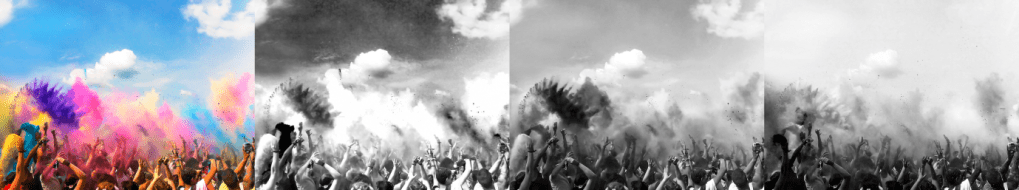
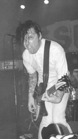
Take a picture, mirror it, turn it black and white, resize it, remove the blemishes – to humans, the result is still recognisable the same picture (or at least, the same source). We see the colours and the pixels and the shapes, where the computer sees only the hex.

Several perceptual hashing methods exist, and I’ve explored a few of my own thoughts as well. Most of my methods trended towards a grid-based/block-based model, where the source image is broken down to an NxN grid, with functions being performed on each grid square and the results being combined into a single hash value. I looked at histograms, variance, and a few statistical functions. However, I believe that Average Hash (or ahash) generally produces better results than I could achieve – in most cases.

Types of Perceptual Hashing There is a Python library currently maintained call ImageHash, which groups together methods of perceptual hashing. I’ll be referencing this for convenience, but this shouldn’t be taken as preaching the gospel. Each method starts with scaling the image down to a square grid, and converting to greyscale. A summary of methods is below.

ahash: take an average pixel value of the whole of the new image and assign a 0 or 1 to each grid square based on whether it is above or below that average.
phash: perform a discrete cosine transform and then use the lowest frequencies as a basis for an ahash-like process.
whash: the same as phash, but using wavelet decompose instead of a DCT (interesting read).
dhash: based on the gradient between proximate pixels.

According to authors of the Python library, ahash performs the worst when searching for similar, not identical, images. Nevertheless, I chose ahash as a basis for a bit of work/play.

How to Perceptually Hash

I would call the first stage of this process “image preparation”. There are too many image formats, and each has their own standards and quirks. The ideal starting point for ahash is a three-channel-per-pixel map of the content, but that’s not how most formats work, so the image must be converted into a matrix, with colour values from 0 to 255 per channel. Alpha channels can be discarded or otherwise handled (provided that method id consistent).

The range should then be stretched so that all values from 0 to 255 are used. Why? This could be an arbitrary step in my implementation, though it should be noted that one thumbnail I created was a perfect match only after stretching the contrast. If used, the interpolation method must be set across all organisations using the same hash sets, or the accuracy of results would suffer – discarding or rounding values at this stage may produce significant variations later in the process.

Three different desaturation methods (original image: andessa)

At first, I used PIL’s function out of simplicity, but then later explored weighted channel mixing. There was a minor difference in which images appeared as false positives, but nothing I found to be significant in the highly similar (>90%) rated images. A test image where I had shifted the hue ±180° was computed as 96.9% similar to the original hash, illustrating that an ahash value is still fairly colour-agnostic.

That’s one reason to convert to grayscale – colour adjustment of duplicates can be mostly ignored. If you kept the data from 3 colour channels, you’d have to do some clever thinking to identify an image with the hue shifted, for example, 40°. Additionally, the hash would be longer by the multiple of the number of channels; in practice, 192 bits rather than 64 bits for 3-channel images (see next section for why 64 bits). I suggest a possible compromise at the end.

I would recommend to the digital forensic community that if perceptual hashing is implemented on a large scale that the conversion method is mathematically defined rather than relying on a specific library or tool. This means cross-language and cross-platform consistency.

The image now needs to be scaled to the chosen size. The size itself is something that bears discussion: I found with my own methods that when comparing the accuracy over grid sizes N=3 to N=10 a grid of N=5 produced the highest contrast between true positives and true negatives, but also computed some similar images as less similar than other N values. I haven’t done sufficient analysis on grid size’s effect on ahash and related functions, but I have noted something about resizing algorithms when I wrote my own ahash function in Python and again in C#. I used the PIL library (Pillow fork) in Python and the inbuilt Image library in C# and my hash values for the same image came out different from each function.

Looking into this, I found that the default methods for resizing were not the same. So naturally, I fixed my code with a simple change of forcing each implementation to use bilinear interpolation. Different hash values again… I’ll admit I could have written their core functions differently, but I concluded after a lot of head-table interaction that the implementation of the interpolation in each library was different. Again, I believe a mathematical definition should be used to standardise the method, though I have not tested, for example, centre-weighted average of pixel values versus weighted brightness, or modal value versus mean value. All of my testing from this point was using PIL’s bilinear resizing, as it seemed to give the most accurate results (subjective).

Most of my testing was conducted on an N=8 grid (which is the same is the ImageHash library), meaning a 64-bit binary string, or a 16-character hex string.

How to Compare Hashes

Yes, this is issue in itself. The simplest method is the same as with cryptographic functions: is hash A identical to hash B? With this, it should be possible to identify identical images within a dataset. Thumbnails aren’t necessarily as easy as that, though, as they likely add another layer of compression and artefacts to the original image. Identifying edited/manipulated images would be impossible.

A perceptual hash is something you compare against, yes, but it is also a map – and I’ll go so far to say a magical map. To illustrate this, I took a test image and overlaid the centre third with the word “FORENSICS” in bold Impact font.

A straight comparison and this would immediately fail – 0% match, just as bad as a cryptographic hash. A comparison of each positional character though, and calculating a “similarity” rating, produces results with more leeway. The edited image ahash now shows 9/16 (56%) similarity.

Original:                0x00003e3e1e1e1e0e
Edit:                    0x00001c7e7f1e0e06

Decomposing the hex string back to the original binary show this:

Original:  0000000000000000001111100011111000011110000111100001111000001110
Edited:    0000000000000000000111000111111001111111000111100000111000000110

This gives a similarity of 56/64, or 87.5%, which is a lot better. But introducing margins like this increases the probability of false positives, right?

Comparing this to a set of 8,089 pictures sourced from a dataset website, the highest similarity to the original came out at 90% similar, and only 3 images were categorised being as similar as or more similar than the “forensics edit”. That’s 0.04% (four one-hundredths of a percent) – I have tested other images with the same technique and this is at the better end; the poorer performing instances identifying up to ~1.5% of the dataset.

What I’ve done to this image introduces more “encoding artefacts” than simply thumbnailing it, and is similar to what some social media apps do. And comparing thumbnails to the originals would be boring – all of the 10 images I thumbnailed were computed at >98% similar.

So perceptual hashes don’t produce a binary result, a yes or a no (at least in my implementation). That’s kind a long walk back to the name of the method – perceptual. Were digital practitioners or organisations to use a perceptual hash library, they would also have to set acceptable and unacceptable similarity ratings for dataset results. This could vary on a case by case basis, or the time investment/risk could be managed at a departmental (or higher) level. Based on my small 8k image dataset, if I were creating a review tool, I would set the global lower limit of similarity at around 85% and a “good match” level at around 98%.

Autobots, Roll Out

It all falls down when you transform an image. The lowest similarity between the source ahash and target ahash I encountered after rotation was 50%, using the above decomposition comparison. That’s worse than many false positives.

However, we see the magic of this map when the hash is partially decomposed to pairs (e.g. 0xC3) or fully decomposed into binary (e.g. 011010…). Since the hash is computed from a square grid of known size, we can perform matrix transformations, or perhaps more easily, slices on the binary string.

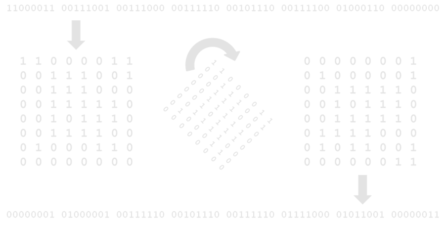
Slicing can be used to determine the perceptual hash of a mirrored image by reversing each “row” (for horizontal) or “column” (for vertical) of data.

With minimal processing power (because of the size of the hash), the hash of all transformed images can be computed, including mirrored and rotated (in increments of quarter turns). Simple transformations of stretching or compressing in the x or y directions require no matrix manipulation, but skewing might be approachable by shifting the sequence a bit or two – this is fairly uncommon though.

Depending on which resources are more readily available, either a database could contain all transformation permutation hash values, or the checking algorithm performs these matrix permutations on each image it processes (regardless, image review software would have to store and index all values for the images being reviewed).

When I had coded this “matrix permutator”, I tested it on a set of rotated and transformed versions of an original image, and found it had a 100% match rate to the original image. I should state at this point, I mean in image editing software that re-encodes the image on saving. Including transformations in the matching model will (almost certainly) increase the number of false positives in a dataset by a factor equivalent to the number of permutations.

Similar Images

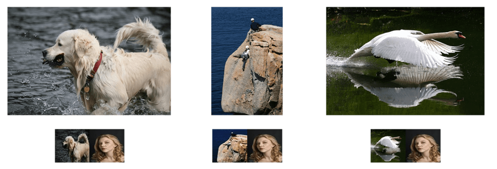
In this context, I mean non-identical images with extremely high content correlation, as below. This similarity is… similar to the above, but I categorise it differently, as the above set features modified images, and this set features unique images.

While we as humans know this is not the same image, we can see the composition and content is beyond similar. My implementation of ahash knows this too – 86% similarity. In the interest of full disclosure though, 11 images from the dataset were computed at ≥86%, including the below.

Again, this is a best case scenario. Heavily manipulated images, or images in a set (such as a photographic series), were not consistently identified by this implementation of ahash – that is, a large quantity of different images were rated as more similar than two from the same set. I would argue that ahash is not well suited to this kind of identifying similarity, but can be used to aid in human-lead identification.

Additional Considerations

Centre Cropping

Mobile phone galleries like to use square cropping to show thumbnail previews of images – hash values produce from the full aspect ratio image could differ significantly from square-cropped images.

I tested one instance each of a ~30% and ~15% crop, which computed to a 66% and a 58% similarity respectively. At this time, I can think of no better solution than centre-cropping the image and storing the ahash value alongside that of the full image.

Colour Matching

The conversion to greyscale is discussed above, but the information discarded at this step may be useful. I have found one method which when used as a supplement to ahash increases result accuracy (for non-colour-shifted images) while using fewer bits than a full colour ahash. This method is almost identical in implementation, but bases the 1 or 0 value on whether the red channel has a higher value than the green channel.

I haven’t fully explored combining this with the main ahash result, but it is clear that using only this metric is not at all suitable. A somewhat convoluted implementation of this metric was able to reduce false positives compared to ahash alone, while still capturing true positives. It does however, and somewhat obviously, fail to identify hue-shifted images.

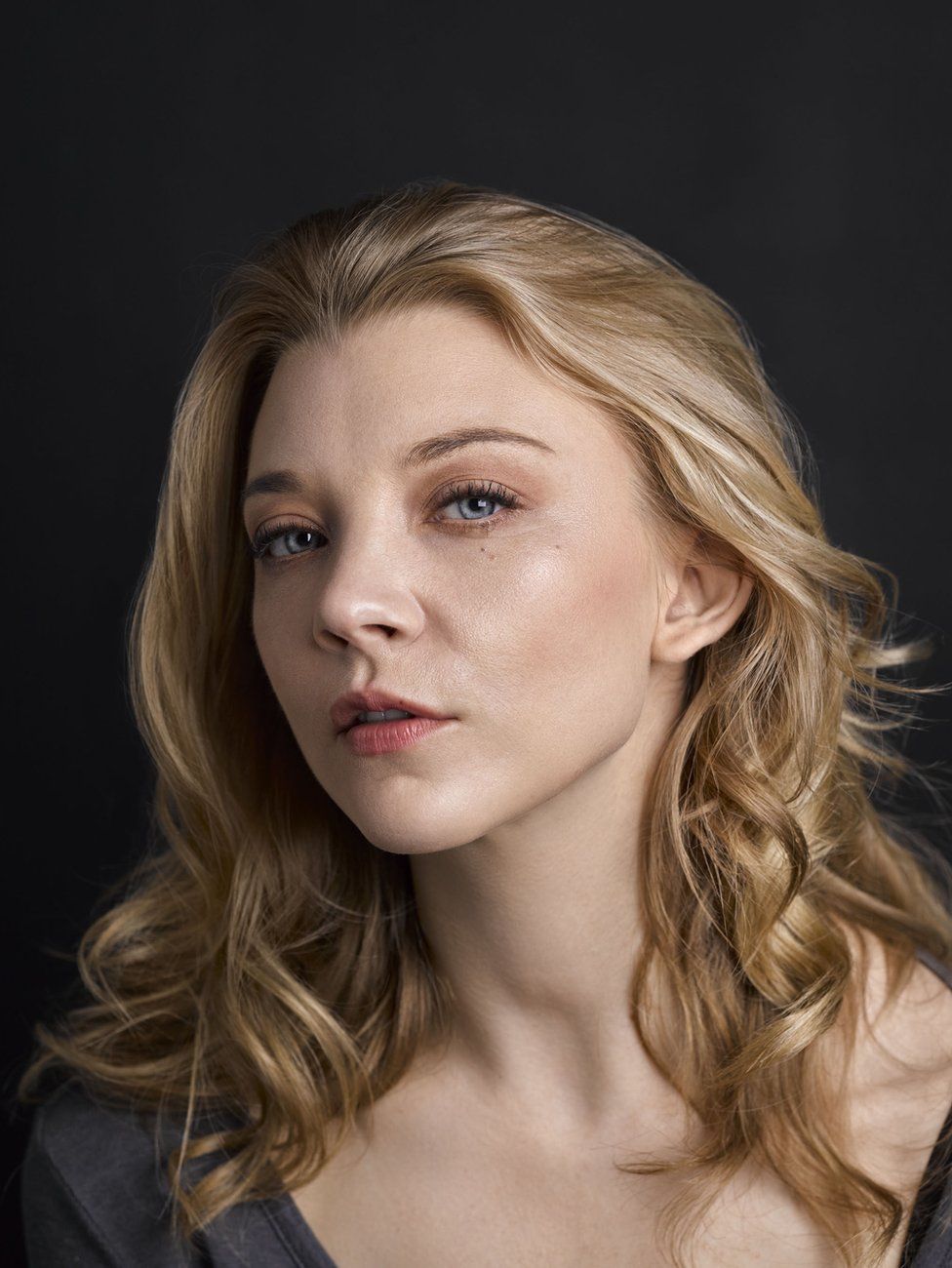
If the ahash similarity is limited to a minimum 85% for a match and this new metric is limited to >98%, the number of false positives have been reduced by up to 70% in my testing. For the image of Natalie Dormer, false positives were reduced from 10 to 4, while still identifying the second Dormer image and thumbnails.

Grid Size

You might imagine that increasing the grid size geometrically increases processing time. This was not the case when I increased grid size from N=8 to N=16 – processing time only increased by a measly 6%, so the bottleneck in my case was the image loading and processing (“preparation”), not the hash computation.

Some images computed as more similar, some as less similar. In this particular dataset, one image was above 85% similar to the Dormer image compared to the 10 when N=8. This is not proof that higher N values are more accurate – more work would have to be done in this area to find optimal grid size.

Dataset

I found my dataset online, and this is not necessarily representative of the images recovered as part of a digital investigation. The thresholds I have mentioned above are in relation to this dataset, and deciding limits for the real world should be informed by real world data.

For reference, here are two plots showing image similarity in the dataset to a chosen image.

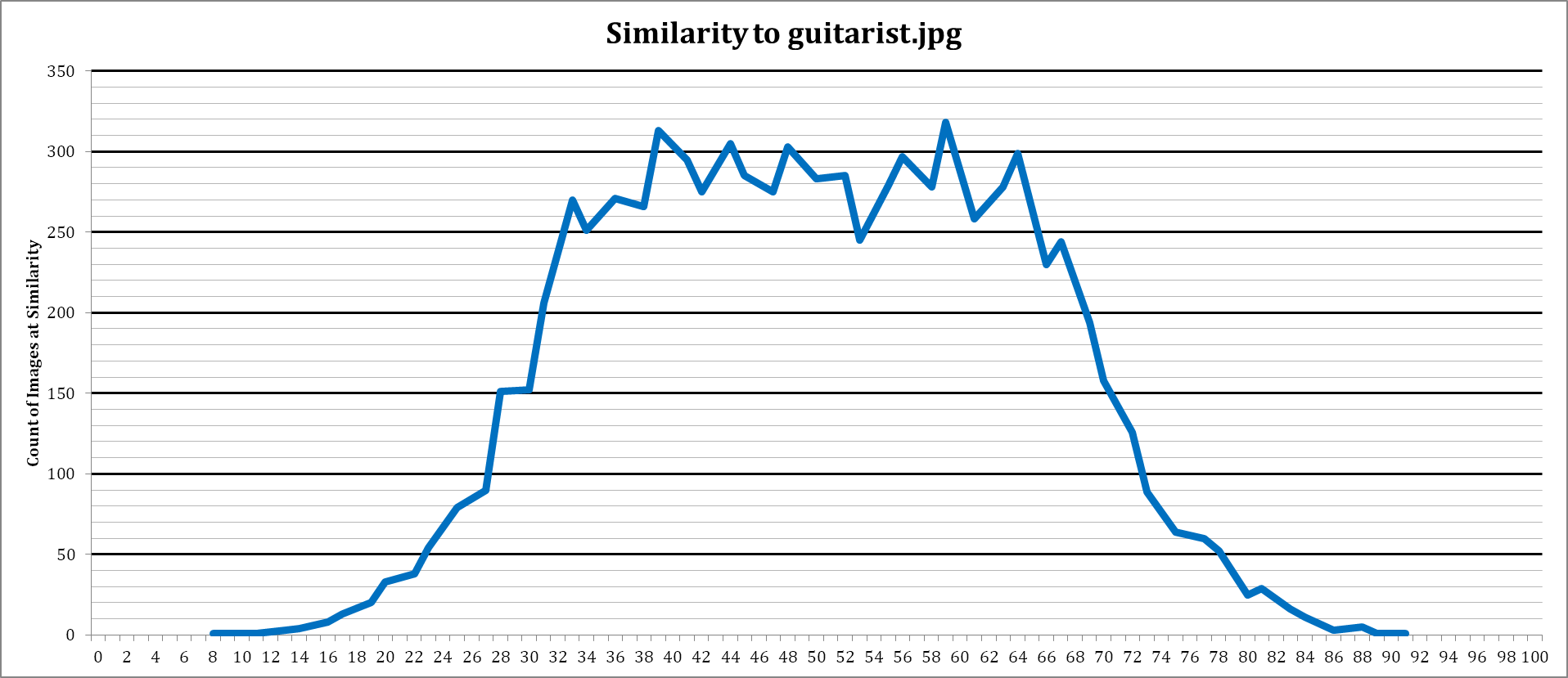
There are both trending towards a normal distribution, but even the difference between the two suggests the dataset is not truly random. Something to consider about this dataset as well, is that it is a collection of photographs – what people thought it was important to capture and preserve, then uploaded to the internet. Real world datasets will contain images from web caches, adverts, and other non-photographs too.

Final Word

Well, that’s a quick look into perceptual hashing. Can it be used to identify visually identical images? Absolutely. Can it be used effectively in digital forensics? There are pitfalls for each perceptual hash method, and a lot of things to consider when setting up your version of it. Using ahash is simple enough that any department or organisation should be able to implement a system without going to an outside company or service and being charged for smart image matching software. Perceptual hashing is fixed, so probably can’t stand up to well-trained AI, but there is a place for it – it’s simple, consistent, and doesn’t require special or expensive hardware.

A database can be set up, much like CAID, that holds the ahash values of images we want to identify. Decomposing stored hashes is no strain on processors, so comparing a new set of images to this database should be just as fast as comparing MD5 values. Computation time to obtain the perceptual hash value may be marginally more, but provides more information. You can get false positives, just like in keyword searches, but reviewing results manually should be very quick – the human brain is good at that sort of thing.

Perceptual hashing could aid in review of material, depending on the area of interest, and is simple enough that it could be used in a volume-based approach, where, for example, investigating officers are reviewing data extractions rather than a digital investigation unit.

I can’t tell you if you should implement perceptual hashing, or exactly how to do so to best suit your needs – you need to implement what you perceive to be the best option.